You need a 1D tolerance stack-up for an assembly gap, clearance, or end-play loop — worst-case for guaranteed fit, RSS for high-volume statistical risk, plus Cp/Cpk and which dimensions drive the variance. This pad lets you add 2–12 dimensions with loop direction (+/−), nominal, and asymmetric +tol/−tol, set LSL/USL and sigma factor k, then returns WC and RSS bands, adjusted RSS with a 1.5σ mean-shift, capability, scrap %, pass/fail, and a contributor ranking.
Defaults open on Metric with a four-part fixture loop: Housing +50 ±0.05, Shaft −49.6 ±0.04, Shim −0.2 ±0.02, End play −0.1 ±0.01 mm, LSL 0, USL 1, k = 3. CALCULATE returns nominal gap 0.10 mm, WC −0.02…0.22 mm (fail), RSS ±0.068 mm → 0.032…0.168 mm (pass), Cpk ≈ 1.47, and Housing ~54% of variance. Switch to Imperial for the inch example. Math stays in your browser.
It sits under Fixture & Tooling Calculators next to the ISO 286 tolerance calculator and GD&T fit calculator. This pad is a linear 1D chain — not Monte Carlo, 2D/3D stacks, or GD&T bonus translation.
Formula
- Nominal gap = Σ (dirᵢ × nominalᵢ) with dir = +1 or −1.
- Statistical mean = Σ dirᵢ × (nominalᵢ + (t+ᵢ − t−ᵢ)/2) for asymmetric zones.
- Worst-case: direction-aware extremes → WC min/max around the nominal gap.
- ti = (t+ᵢ + t−ᵢ)/2; σᵢ = ti/k; σasm = √Σσᵢ²; RSS@k = k·σasm (= √Σti² when all use the same k).
- Adjusted RSS (1.5σ shift) = (k + 1.5)·σasm about the statistical mean.
- Cp = (USL − LSL)/(6σasm); Cpk = min(USL−μ, μ−LSL)/(3σasm); scrap % from normal tails outside LSL/USL.
- Contributor %ᵢ = σᵢ² / Σσⱼ² × 100.
Reproduce the default Metric loop on CALCULATE:
| Quantity | Value |
|---|---|
| Inputs | +50±0.05 · −49.6±0.04 · −0.2±0.02 · −0.1±0.01 · LSL 0 · USL 1 · k=3 |
| Nominal gap | 0.10 mm |
| Worst-case | −0.02 … 0.22 mm → FAIL |
| RSS 3σ | ±0.0678 mm → 0.032 … 0.168 mm → PASS |
| Cp / Cpk | ≈ 7.37 / 1.47 |
| Top contributor | Housing ≈ 54% variance |
How it works
Build a 1D dimension loop with direction, nominal, and +/- tolerances. Worst-case adds arithmetic extremes. RSS combines independent normal variation at your sigma factor k (tolerance = +/-k sigma). Adjusted RSS adds a 1.5 sigma mean-shift. Cp/Cpk and scrap % use the assembly sigma against your LSL/USL. Contributor % ranks which dimensions drive stack variance.
Pick Metric or Imperial (tab switch resets defaults). Set LSL/USL and sigma factor k (tolerance = ±kσ). Add or remove loop rows (2–12): label, direction (+ adds / − subtracts), nominal magnitude, +tol and −tol. CALCULATE fills Results (gap spectrum, WC/RSS/adjusted RSS, Cp/Cpk, scrap %, contributor table). Editing a field clears Results. RESET restores the active tab’s fixture-loop defaults.
Worst-case vs RSS — when each method wins
Shop tolerance stack-up tools all report both arithmetic worst-case and root-sum-square. Worst-case assumes every dimension sits at its most unfavorable limit at once — WC = Σ|ti| in the closing sense. RSS assumes independent, centered, normal variation: RSS = √Σti² when each drawing tolerance is treated as ±kσ.
RSS is always tighter than (or equal to) worst-case for the same stack. Use worst-case for safety-critical or low-volume builds that must assemble every time. Use RSS for high-volume production when process data supports statistical treatment — and still review worst-case at design gates where guaranteed fit matters.
Default four-part loop (mm, k = 3):
| Method | Band | vs LSL 0 / USL 1 |
|---|---|---|
| Worst-case | −0.02 … 0.22 | FAIL (min < 0) |
| RSS 3σ | 0.032 … 0.168 | PASS |
| Adjusted RSS (4.5σ) | −0.002 … 0.202 | FAIL (min < 0) |
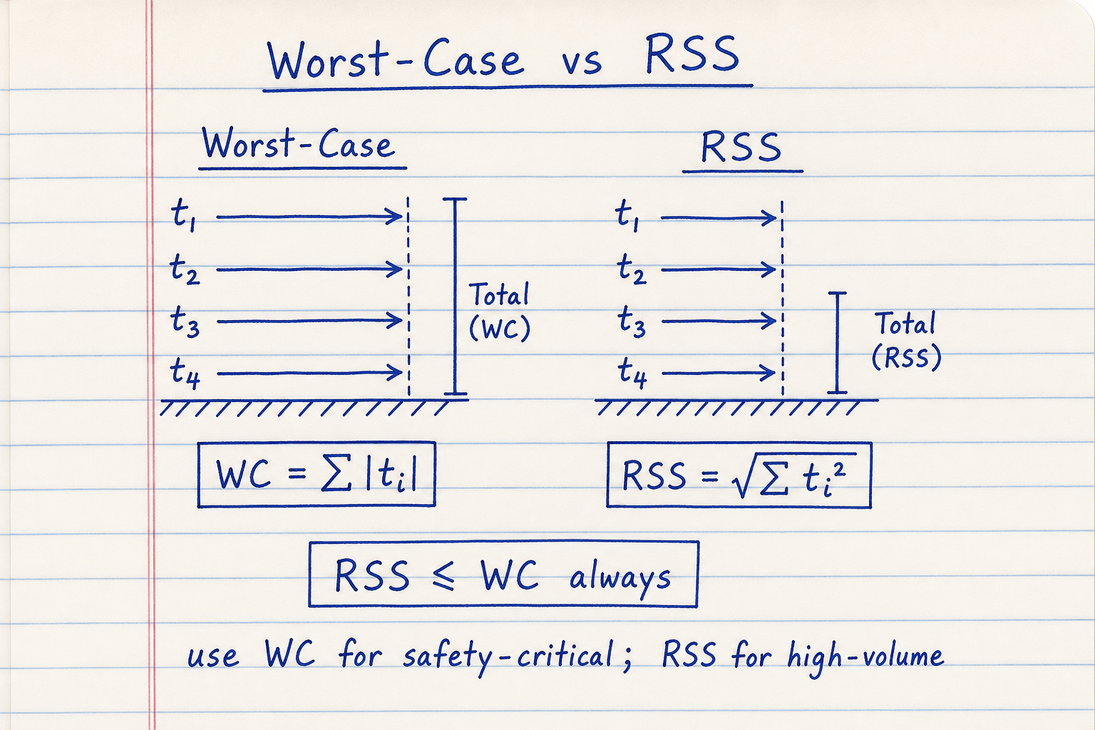
Default CALCULATE path: WC half-width 0.12 mm vs RSS ±0.068 mm — RSS is ~43% tighter.
If an older pad showed RSS larger than WC, the sigma factor was double-counted; this pad uses RSS = √Σti² at the chosen k.
Loop direction — building the functional chain
Tolerance stack-up guides start the same way: define the point of interest (gap, clearance, end play), mark a positive direction, then walk part-to-part along one functional path. Each dimension gets a + or − sense in that loop.
On this pad, nominals are magnitudes and Direction sets the sign. +50 with −49.6 −0.2 −0.1 is the same gap as the classic signed sum 50 − 49.6 − 0.2 − 0.1. +Tol / −Tol are drawing tolerances on that feature; worst-case maps them through direction so a larger shaft (when the shaft subtracts) correctly closes the gap.
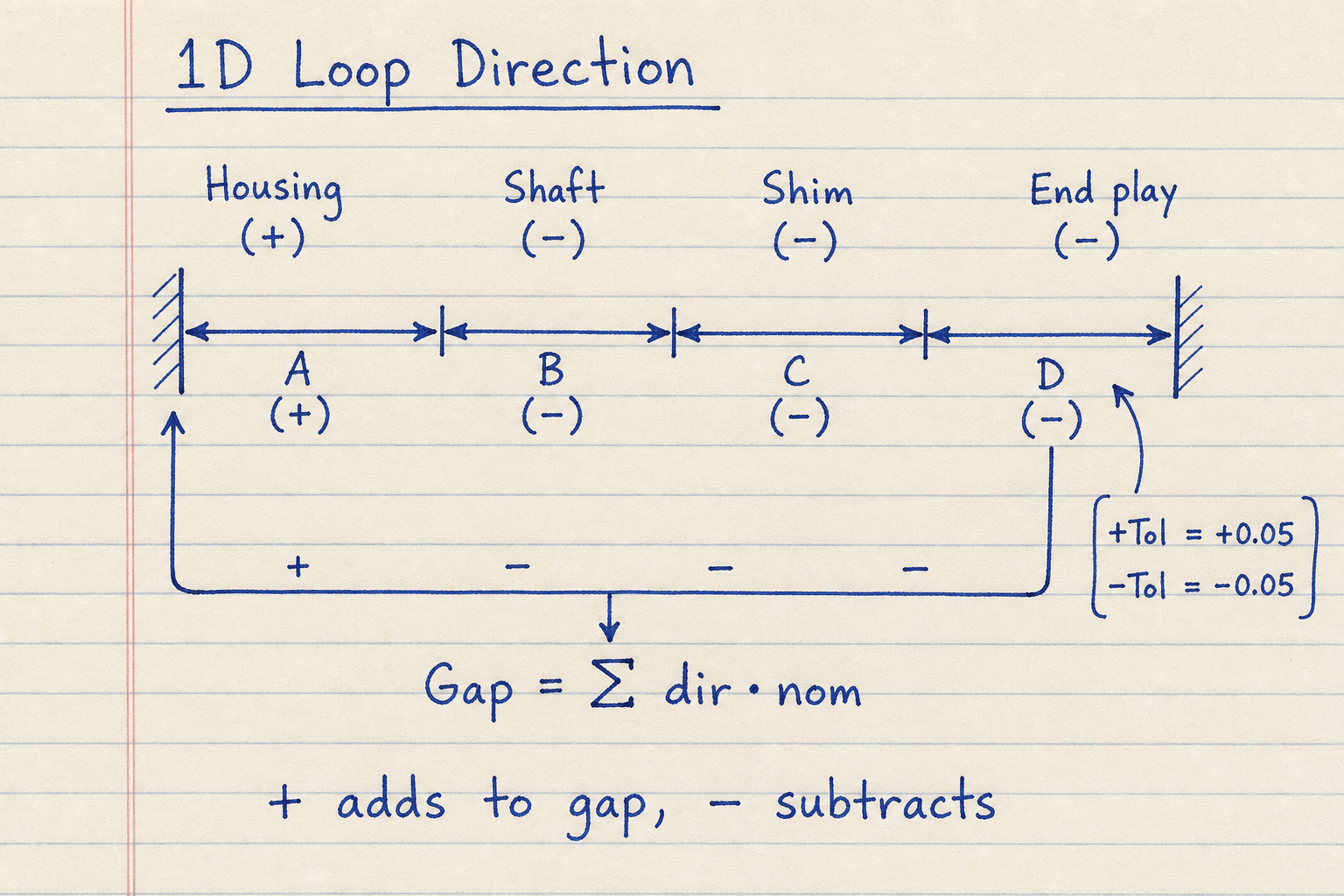
Typical chains run 3–10 dimensions; this pad allows 2–12. Enter +Tol and −Tol as positive magnitudes (the UI does not use a signed −Tol field).
Keep one consistent unit system for the whole loop — Metric and Imperial tabs reset defaults so you do not mix mm and inches.
Cp, Cpk, scrap, and contributor ranking
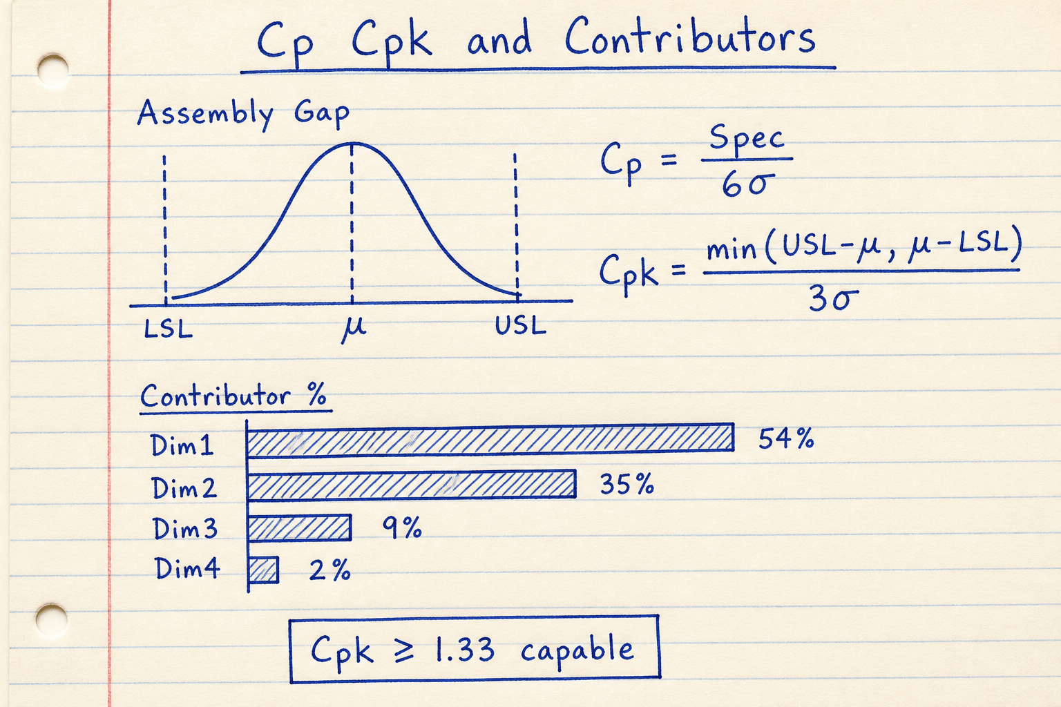
Once σasm is known from RSS, capability is the same language as process control: Cp compares the full specification width to 6σ; Cpk also checks centering. A Cpk of 1.33 or higher is a common “capable” gate. Scrap % estimates the normal-distribution tails outside LSL/USL — useful for production risk, not a substitute for Monte Carlo when distributions are skewed or correlated.
Contributor % is each dimension’s share of assembly variance (σᵢ² / Σσⱼ²). Tighten the top contributors first — on the default loop, the housing ±0.05 drives about 54% of the stack variance, so shaving that band moves Cpk more than chasing the 0.01 end-play.
Default contributor share (k = 3):
| Dimension | ti (mm) | % variance |
|---|---|---|
| Housing | 0.05 | 54.3% |
| Shaft stack | 0.04 | 34.8% |
| Shim | 0.02 | 8.7% |
| End play | 0.01 | 2.2% |
Adjusted RSS widens the statistical band by a 1.5σ mean-shift (Six Sigma-style drift) — common in tolerance-analysis worksheets next to plain RSS.
Monte Carlo and multi-module GD&T stacks (clearance-hole, datum shift) stay out of scope; use dedicated tools when the loop is non-linear.
Worked example
Four-component Metric fixture loop with k = 3 and gap requirement 0…1 mm.
- Nominal gap = +50 − 49.6 − 0.2 − 0.1 = 0.10 mm
- WC = 0.10 ± 0.12 → −0.02 … 0.22 mm → fails LSL
- ti = 0.05, 0.04, 0.02, 0.01 → RSS = √Σti² ≈ 0.0678 mm
- RSS band 0.032 … 0.168 mm → passes; Cpk ≈ 1.47; Housing ≈ 54% variance
Result: Worst-case fails; RSS passes. Tighten housing or redesign before relying on statistical assembly.
When to use
- Checking assembly gap, clearance, shim, or end-play in a 1D dimension loop
- Comparing worst-case vs RSS (and adjusted RSS) before releasing drawings
- Ranking which tolerances to loosen or tighten for cost vs capability
- Estimating Cp/Cpk and scrap risk when process data supports normal RSS
Limitations
- 1D linear chains only — not 2D/3D stacks, thermal growth, or deflection
- RSS assumes independent, random, reasonably centered normal contributors
- No Monte Carlo; adjusted RSS is a 1.5σ mean-shift envelope, not a full simulation
- Does not translate GD&T modifiers, bonus tolerance, or datum shift into linear ti
FAQ
- Worst-case vs RSS?
- Worst-case adds every tolerance at its most unfavorable extreme — conservative and required when every assembly must fit. RSS combines independent normal variation as √Σti² and is typical for high-volume production with capable processes. RSS should never exceed worst-case for the same stack.
- What sigma factor k should I use?
- k = 3 is the usual assumption (drawing tolerance ≈ ±3σ). The RSS band at that k is √Σti². Raise k only when your process data says the tolerance band covers more than 3σ.
- What are Cp and Cpk here?
- They treat the assembly gap as a process with σ = σasm from RSS. Cp = (USL−LSL)/(6σ); Cpk also accounts for mean location. Cpk ≥ 1.33 is a common capable threshold. Scrap % is the estimated normal-distribution fail rate outside LSL/USL.
- How many dimensions should I include?
- Include every dimension on the functional path from one side of the gap to the other. Typical loops are 3–10 dimensions; this pad allows 2–12. Skip unrelated features that do not sit in the chain.
ISO 286 Tolerance Calculator
ISO 286 hole/shaft limits, deviations, and clearance / transition / interference fit type.
Open calculatorGD&T Fit Calculator
Shaft-hole MMC/LMC clearance, fit type, and optional virtual-condition go-gauge envelopes.
Open calculatorLocating Pin Fit Calculator
Pin–hole clearance, transition, or interference from ISO-style deviations, plus Lamé press-force screening.
Open calculatorGauge R&R Calculator
MSA Gauge R&R from Xbar-R summary or EV/AV/PV: %GRR vs tolerance and study variation, NDC, AIAG status.
Open calculator